Adventures in Reinforcement Learning

Just recently my son wanted to program a game for his school computing project.  After several rounds of discussion where I convinced him on the challenges of P2P socket programming along with game state management as well as the fact that he had to rely on himself to do most of the work (not me! 😂); that we settled on a simple turn based Othello game.

So what I did was to first code up the whole game myself to get a sense of the complexity as well as the programming topics I would need to teach my son about (e.g. data structures, game play, algorithm design, GUI event model etc …); so that I will be able to guide him as he codes up the game.

Simple turn based GUI for Othello game using Turtle graphics

I managed to code up a simple turn based game in Python using Turtle graphics.  It was a fun project and it allowed me to exercise my coding muscles.  But I thought to myself, can I bring this one step further?  It turns out, I can.

I took this opportunity to extend the project to training a reinforcement learning agent to play Othello.  Eventually, I was able to develop the following:

  1. Custom Gym environment based on the Othello game
  2. DQN agent with simple epsilon greedy policy and replay buffer
  3. Human and Agent game mode for Othello

Usually I would make this into a tutorial on how to build this but seeing that there are a lot of areas to cover, I decided to share the resources and steps that I used to develop this code and hopefully you can do the same as well.


Step 1: Learning about Reinforcement Learning

A great resource that I used to learn about Reinforcement Learning is the Udemy course – Practical AI with Python and Reinforcement Learning. (https://www.udemy.com/course/practical-ai-with-python-and-reinforcement-learning/)

This is a great course that will teach you the basics and theories about Reinforcement Learning together with relevant and useful coding exercises.  I recommend that you pay attention to the following chapters

  1. Reinforcement Learning – Core Concepts
  2. OpenAI Gym Overview
  3. Classical Q Learning
  4. Deep Q-Learning
  5. Creating Custom OpenAI Gym Environments

Step 2: Papers and existing work done with RL for Othello

I found the following papers helpful in deciding the architecture of the DQN agent as well as how the training is to be done.

Step 3: Learn from others

I also found learning from others who have coded similar projects useful to see how they implemented some of the concepts in the papers above.  One good repository is https://github.com/xyqfountain/Othello-Reversi-Env-for-Reinforcement-Learning


My current code is rather simple in that the training is based on Epsilon Greedy Policy together with a basic implementation of replay buffer.  However even with this basic setup, I am able to achieve between 70% to 80% win rate (across 30 games) against an opponent using a random play strategy.

Agent (White player) training in progress with visual game play

You can download my code here – https://github.com/ianlokh/Othello.git which will allow you to train your own agent and even play against it. It is a fun way to assess how well you stack up against the agent.

I will be continually updating this code to explore other RL techniques so please come back for more updates.

That’s all for now and I hope you will find this useful in your RL learning journey!

Classifying Duplicate Questions with TensorFlow

Recently I have been attending the TensorFlow and Deep Learning meetup in Singapore. This is a great group of people who are passionate about Deep Learning and using TensorFlow to solve all kinds of interesting problems. Do join us if you can on Meetups.

I was given the great opportunity to share about applying Convolutional Neural Networks using TensorFlow to try to classify duplicate questions on Quora. This is the same as the Kaggle competition QuoraQuestionPairs.

In this tutorial, I will be walking through the process of generating the text features I used and how to use TensorFlow and TensorBoard to monitor the performance of the model.

All the source code, notebook and keynote presentation can be found at here. A video of my presentation can also be found here.

Lets start!

Problem Description

In the Kaggle problem, we are to build a classifier that will determine if two questions are identical based on a (human) labelled dataset. In this dataset the only information provided is

  • Question IDs
  • Questions pair (Q1 and Q2)
  • Is Duplicate label (0, 1)

The key evaluation criterion is log-loss but for this tutorial, we will be considering the usual metrics for classifications in addition to the log-loss metric to evaluate performance.

In order to keep this tutorial brief, we will not be covering the usual EDA activities and jump straight into feature generation, modeling and model evaluation.

Please note that this is by no means all the features you should be generating. The general idea is that the more features the better – but you would need to pay attention to the specific features to be used.

Feature Generation

Note: refer to “qqp_BaselineModels.py”

Word & Character Counts

The first set of features we will build are word and character counts of each of the questions. The naïve intuition is that questions that are similar to each other would likely to have similar sentence structure and hence word counts.

# get count of words in each question
def word_count(df, dest_col_ind, dest_col, src_col):
    df.insert(dest_col_ind, dest_col, df.apply(lambda x: len(x[src_col].split(' ')), axis=1, raw=True))
    return df

df_all = applyParallel(df_all.groupby(df_all.grpId), word_count, {"dest_col_ind": df_all.shape[1]-1,
                                                                  "dest_col": "tr_q1WrdCnt",
                                                                  "src_col": "q1nopunct"}, _cpu)  

The code above uses the function applyParallel to parallelize the word count function over rows in the dataset. You can refer to my previous post on how this works here. The same code structure is also used to generate the character count.

Depending on your approach, you can also normalize the counts – generally if you are using XGBoost, normalization may not be as important as binning. However for NN based models, it is generally advisable to normalize so that their effects do not overwhelm the other features.

Share of Matching Words

The next set of features is based on the general idea that if two sentences share similar words they should be closely related or duplicates. The higher the percentage of matching words, the more likely they are duplicates.

def word_match_share(df, dest_col_ind, dest_col, columnname1, columnname2):
    df.insert(dest_col_ind, dest_col, df.apply(lambda x: utils.word_match_share(x, columnname1, columnname2), axis=1, raw=True))
    return df

df_all = applyParallel(df_all.groupby(df_all.grpId), word_match_share, {"dest_col_ind": df_all.shape[1]-1,
                                                                        "dest_col": "wrdmatchpct",
                                                                        "columnname1": "q1nopunct",
                                                                        "columnname2": "q2nopunct"}, _cpu)

TF-IDF Weighting

Another set of features can be generated using TF-IDF weighting. The use of TF-IDS is based on the intuition that common words across the corpus (all the questions) will be less important hence given a lower weightage and conversely, uncommon words across the corpus have more information content and hence will be given a higher weightage.

This means that questions with unique terms that appear in one question and not the other are thus less likely to be duplicates.

We first create the TF-IDF vectorizer using the questions as the input corpus.

# create corpus for tfidf vectoriser
corpus = df_all['q1nopunct'].append(df_all['q2nopunct'], ignore_index=True)

# create tf-idf vectoriser to get word weightings for sentence
tf = TfidfVectorizer(tokenizer=utils.tokenize_stem,
                     analyzer='word',
                     ngram_range=(1,2),
                     stop_words = 'english',
                     min_df = 0)

# initialise the tfidf vecotrizer with the corpus to get the idf of the corpus
tfidf_matrix =  tf.fit_transform(corpus)

# using the source corpus idf, create the idf from the input text
tfidf_matrix_q1 =  tf.transform(df_all['q1nopunct'])
tfidf_matrix_q2 =  tf.transform(df_all['q2nopunct'])

Next we convert the sparse matrixes into dataframes and determine the sum and mean. We do this for both questions.

#Converting the sparse matrices into dataframes
transformed_matrix_1 = tfidf_matrix_q1.tocoo(copy = False)
weights_dataframe_1 = pd.DataFrame({'index': transformed_matrix_1.row,
                                    'term_id': transformed_matrix_1.col,
                                    'weight_q1': transformed_matrix_1.data})[['index', 'term_id', 'weight_q1']].sort_values(['index', 'term_id']).reset_index(drop = True)

sum_weights_1 = weights_dataframe_1.groupby('index').sum()
mean_weights_1 = weights_dataframe_1.groupby('index').mean()

Word2Vec Embeddings

Note: refer to “qqp_BaselineModels.py” and “img_feat_gen.py”

To generate the embeddings for each pair of words between the two questions, Gensim’s implementation of word2vec was used with the Google News corpus. For each pair of words, the similarity score is determined and used to create a 28 x 28 matrix. The 28 x 28 matrix is then visualised to have a sense of whether the similarity scores contain information that will help with the classification.

    df = applyParallel(df.groupby(df.grpId), ifg.gen_img_feat, {"dest_col_ind": df.shape[1]-1,
                                                                "dest_col_name": "28_28_matrix",
                                                                "col1": "q1nopunct",
                                                                "col2": "q2nopunct",
                                                                "matrix_size": 28,
                                                                "order": 0,
                                                                "show": False,
                                                                "tofile": False}, _cpu)
    print("Finished gen_img_feat processing", str(i), "chunks")
  • This function is placed in a loop that chunks the training dataset for processing because of memory constraints.
# 2) Create a matrix between the similarity score of both questions and visualise it
def to_image(row, col1, col2, matrix_size, order, show=False, tofile=False):
    if (utils.is_nan(row[col1]) == True):
        c1tokens = []
    else:
        c1tokens = list(map(lambda x: x.lower(), utils.tokenizer(row[col1])))

    if (utils.is_nan(row[col2]) == True):
        c2tokens = []
    else:
        c2tokens = list(map(lambda x: x.lower(), utils.tokenizer(row[col2])))

    score = [word_word_score(a, b) for a, b in itertools.product(c1tokens, c2tokens)]
    # for questions with null values, score will be empty array so need to preset value to 0.0
    if (len(score) == 0):
        score = [0.0]
    arr = np.array(score, order='C')
    # determine the current dimensions
    #arrsize = len(arr)
    length = math.ceil(math.sqrt(len(arr)))
    # create matrix based on current dimension
    img = np.resize(arr, (length, length))
    #print('Row: {0}, Orig matrix length: {1}, Sqrt: {2}, Zoom: {3}'.format(row["id"], arrsize, length, ((matrix_size**2) / (length**2))))

    # zoom the matrix to fit 28 x 28 image
    img = scipy.ndimage.interpolation.zoom(img,
                                           #((matrix_size**2) / (length**2)),
                                           (matrix_size / length),
                                           order = order,
                                           mode = 'nearest').round(5)

    if (row['grpId'] == 0):
        if show:
            display = img
            # print img
            #fig = plt.figure()
            # tell imshow about color map so that only set colors are used
            display = plt.imshow(display, interpolation='nearest', cmap=cm.coolwarm)
            # make a color bar
            plt.colorbar(display)
            plt.grid(False)
            plt.text(0, -3, 'Is Dup:{0}'.format(row['is_duplicate']), ha='left', rotation=0, wrap=True, fontsize=10)
            plt.text(0, -2, 'Q1:{0}'.format(row[col1]), ha='left', rotation=0, wrap=True, fontsize=10)
            plt.text(0, -1, 'Q2:{0}'.format(row[col2]), ha='left', rotation=0, wrap=True, fontsize=10)
            if tofile:
                plt.savefig('./img/img_{0}'.format(row['id']), dpi = 100)
            else:
                plt.show()

            plt.clf()
            plt.cla()
            plt.close()
            #print('Orig matrix length: {0}, Sqrt: {1}, Zoom: {2}'.format(arrsize, length, ((matrix_size**2) / (length**2))))
            #print('New matrix length: {0}, Sqrt: {1}'.format(len(img.flatten()), math.ceil(math.sqrt(len(img.flatten())))))

    # important to set the return as a list
    return [img.flatten()]

The “to_image” function will call the Gensim word2vecmodel.similarity to get the similarity score and if the matrix is smaller than 28 x 28, a zoom will be applied to scale it up to 28 x 28.

WordNet Similarity Scores

Note: refer to “wordnetutils.py” – It took about 3 days to generate the scores for the entire training and test data questions, so I strongly do not recommend you run this on your laptop / desktop. Which is why I have provided a small subset of the scores in the “df_all_train_pres.h5” file. In this file, the similarity scores for each pair of questions for each training case has been generated.

The next set of features generated are similarity scores based on WordNet. WordNets is a large database of words that are grouped into sets of cognitive synonyms (synsets), each expressing a distinct concept. Synsets are interlinked by means of conceptual-semantic and lexical relations. The resulting network of meaningfully related words and concepts.

We use this database to score how close / apart the meaning of each word in both questions as an approximation to semantic similarity. You can find the original code and approach here. Credit goes to Sujit Pal.

Up to this point in the tutorial, we have generated all the necessary features for our model. For simplicity and convenience of this tutorial, the file df_all_train_pres.h5 has been created so that we can proceed with the next step which is to build the CNN model.

Building the CNN Model

Note: refer to “qqp_TensorFlowCNN_Model.py”

Convolutional Network

We begin by reading the HD5 file that we have created to persist the features. The benefit of using this is that we do not have to worry about memory constraints as we can chunk the reading if needed. We will skip the loading of the training data and go straight into the CNN modelling.

# -----------------------------------------------------------------------------
# first convolutional layer
with tf.name_scope('layer_1'):
    W_conv1 = weight_variable([3, 3, 1, 32])
    b_conv1 = bias_variable([32])
    # convolve x_image with the weight tensor, add the bias, apply the ReLU function, and finally max pool
    h_conv1 = tf.nn.relu(conv2d(x_image, W_conv1) + b_conv1)

    # The max_pool_2x2 method will reduce the image size to 14x14.
    h_pool1 = max_pool_2x2(h_conv1)

# -----------------------------------------------------------------------------
# second convolutional layer
with tf.name_scope('layer_2'):
    W_conv2 = weight_variable([5, 5, 32, 64])
    b_conv2 = bias_variable([64])
    h_conv2 = tf.nn.relu(conv2d(h_pool1, W_conv2) + b_conv2)

    # The max_pool_2x2 method will reduce the image size to 7x7.
    h_pool2 = max_pool_2x2(h_conv2)

# -----------------------------------------------------------------------------
# third convolutional layer
with tf.name_scope('layer_3'):
    W_conv3 = weight_variable([5, 5, 64, 64])
    b_conv3 = bias_variable([64])
    h_conv3 = tf.nn.relu(conv2d(h_pool2, W_conv3) + b_conv3)

    # The max_pool_2x2 method will reduce the image size to 4x4.
    h_pool3 = max_pool_2x2(h_conv3)

# -----------------------------------------------------------------------------
# dense fully connected layer
with tf.name_scope('denselayer'):
    # we add a fully-connected layer with 1024 neurons to allow processing on the entire image
    W_fc1 = weight_variable([3 * 5 * 64, 960])
    b_fc1 = bias_variable([960])
    # We reshape the tensor from the pooling layer into a batch of vectors
    h_pool3_flat = tf.reshape(h_pool3, [-1, 3 * 5 * 64])

    # multiply by a weight matrix, add a bias, and apply a ReLU.
    h_fc1 = tf.nn.relu(tf.matmul(h_pool3_flat, W_fc1) + b_fc1)

# -----------------------------------------------------------------------------
# dropout layer
with tf.name_scope('dropout'):
    keep_prob = tf.placeholder(tf.float32)
    h_fc1_drop = tf.nn.dropout(h_fc1, keep_prob, seed=SEED)

# -----------------------------------------------------------------------------
# readout layer
with tf.name_scope('readout'):
    W_fc2 = weight_variable([960, 2])
    b_fc2 = bias_variable([2])
    y_conv = tf.matmul(h_fc1_drop, W_fc2) + b_fc2

This is a simple CNN model with 3 convolutional layers, 1 fully connected layer, 1 drop out layer and 1 read out layer. Note that for the first layer, the filter shape was 3 x 3 instead of the commonly used 5 x 5.

Also note that instead of a 28 x 28 x 64 fully connected layer , we are using a 3 * 5 * 64 layer because of the non-square matrix (24 x 33) of the input vector due to the number of features we have created previously.

Define Functions

Another important step is the definition of the loss functions, regularizers, optimizers and evaluation functions. This includes setting up the confusion matrix and defining the precision, recall and f-score functions. Note that we are using the tf.name.scope to organise the graph so that we can visualise the flow on TensorBoard.

with tf.name_scope('cross_entropy'):
    # Training computation: logits + cross-entropy loss
    cross_entropy = tf.reduce_mean(tf.nn.softmax_cross_entropy_with_logits(labels=y_, logits=y_conv))

    # L2 regularization for the fully connected parameters.
    regularizers = (tf.nn.l2_loss(W_fc1) + tf.nn.l2_loss(b_fc1) +
                    tf.nn.l2_loss(W_fc2) + tf.nn.l2_loss(b_fc2))

    # Add the regularization term to the cross_entropy.
    cross_entropy += 5e-4 * regularizers

with tf.name_scope('train'):
    # Evaluate different optimizers
    # Optimizer: set up a variable that's incremented once per batch and controls the learning rate decay.
    batch = tf.Variable(0, dtype=tf.float32)

    # Decay once per epoch, using an exponential schedule starting at 0.01.
    learning_rate = tf.train.exponential_decay(0.005,                # Base learning rate
                                               batch * BATCH_SIZE,  # Current index into the dataset.
                                               train_size,          # Decay step.
                                               0.94,                # Decay rate.
                                               staircase=True)

    # Use simple momentum for the optimization.
    #train_step = tf.train.MomentumOptimizer(learning_rate, 0.9).minimize(cross_entropy, global_step=batch)
    #train_step = tf.train.GradientDescentOptimizer(learning_rate).minimize(cross_entropy, global_step=batch)
    train_step = tf.train.AdamOptimizer(1e-4).minimize(cross_entropy, global_step=batch)

with tf.name_scope('evaluation'):
    # evaluation criteron
    correct_prediction = tf.equal(tf.argmax(y_conv,1), tf.argmax(y_,1))
    # calculate accuracy
    accuracy = tf.reduce_mean(tf.cast(correct_prediction, tf.float32))

with tf.name_scope('confusionmatrix'):
    # Compute a per-batch confusion
    batch_confusion = tf.confusion_matrix(labels=tf.argmax(y_,1), predictions=tf.argmax(y_conv,1), num_classes=NUM_CLASSES)

    # Create an accumulator variable to hold the counts
    confusion = tf.Variable( tf.zeros([NUM_CLASSES, NUM_CLASSES], dtype=tf.int32 ), name='confusion' )

    # Create the update op for doing a "+=" accumulation on the batch
    confusion_update = confusion.assign(confusion + batch_confusion )

    # Cast counts to float so tf.summary.image renormalizes to [0,255]
    confusion_image = tf.reshape( tf.cast( confusion_update, tf.float32), [1, NUM_CLASSES, NUM_CLASSES, 1])

    # Count true positives, true negatives, false positives and false negatives.
    tp = tf.count_nonzero(tf.argmax(y_conv,1) * tf.argmax(y_,1))
    tn = tf.count_nonzero((tf.argmax(y_conv,1) - 1) * (tf.argmax(y_,1) - 1))
    fp = tf.count_nonzero(tf.argmax(y_conv,1) * (tf.argmax(y_,1) - 1))
    fn = tf.count_nonzero((tf.argmax(y_conv,1) - 1) * tf.argmax(y_,1))

    # Calculate accuracy, precision, recall and F1 score.
    #accuracy = (tp + tn) / (tp + fp + fn + tn)
    precision = tp / (tp + fp)
    recall = tp / (tp + fn)
    fmeasure = (2 * precision * recall) / (precision + recall)


Define Summaries & Run Model

The final step here is where we define the summaries to be displayed on TensorBoard as well as the training loop for the mini-batch training.

It is important to note that prior to executing the training loop, the statement sess.run(tf.global_variables_initializer())must be executed so that all the variables will be initialised in TensorFlow.

# -----------------------------------------------------------------------------
# Define summaries to display on tensorboard
# create a summary for our cost, accuracy and confusion matrix
# Add metrics to TensorBoard.
tf.summary.scalar('Precision', precision)
tf.summary.scalar('Recall', recall)
tf.summary.scalar('f-measure', fmeasure)

tf.summary.scalar("Error Rate", cross_entropy)
tf.summary.scalar("Accuracy", accuracy)
tf.summary.image("Confusion", confusion_image)

# merge all summaries into a single "operation" which we can execute in a session
summary_op = tf.summary.merge_all()

# create log writer object
writer = tf.summary.FileWriter("./log/qqp", graph=sess.graph)

# initialise variables
sess.run(tf.global_variables_initializer())

# Training model run
for step in range(int(NUM_EPOCHS * train_size) // BATCH_SIZE):
    # Compute the offset of the current minibatch in the data.
    # Note that we could use better randomization across epochs.
    offset = (step * BATCH_SIZE) % (train_size - BATCH_SIZE)
    batch_data = x_trndata.iloc[offset:(offset + BATCH_SIZE)]
    batch_labels = y_trndata.iloc[offset:(offset + BATCH_SIZE)]

    if step%(EVAL_FREQUENCY//10) == 0:
        #train_accuracy = accuracy.eval(session=sess, feed_dict={x:batch_data, y_: batch_labels, keep_prob: 1.0})
        #error = cross_entropy.eval(session=sess, feed_dict={x:batch_data, y_: batch_labels, keep_prob: 1.0})
        summary, train_accuracy, error, bcm = sess.run([summary_op, accuracy, cross_entropy, batch_confusion], feed_dict={x:batch_data, y_: batch_labels, keep_prob: 1.0})
        # write log every EVAL_FREQUENCY//10
        writer.add_summary(summary, step)

        # print every eval_frequency
        if step%(EVAL_FREQUENCY*10) == 0:
            print("step %d, training accuracy %g %g"%(step, train_accuracy, error))

    train_step.run(session=sess, feed_dict={x: batch_data, y_: batch_labels, keep_prob: 0.5})

# Validation of training model run
start = 0
end = 0

for i in range(1, round(len(x_validdata)/BATCH_SIZE)-1):
    #  batch = mnist.train.next_batch(50)
    start = end
    end = i*BATCH_SIZE
    batch = (np.array(x_validdata.iloc[start:end]), np.array(y_validdata.iloc[start:end]))

    if i%EVAL_FREQUENCY == 0:
        test_accuracy = accuracy.eval(session=sess, feed_dict={x:batch[0], y_: batch[1], keep_prob: 1.0})
        print("step %d, test accuracy %g"%(i, test_accuracy))

You should now be able to run this code and I hope that this will give you a kick-start in your coding with TensorFlow

Parallel apply in Python

Often in text analytics, we need to process many sentences as part of the text pre-processing (e.g. stemming, stop word removal, punctuation removal) prior to creating the DTM.

Processing the corpus serially would take quite a long time and often we would use SMP to help speed up the process. One of the most useful functions is the apply functions.

In R, this is relatively simple using parapply or dopar. We would just simply use these in place of the familiar apply family of functions. You can learn more about the apply family of functions from the links below:

However with Python, there is no out-of-the-box implementation of parallel apply. And while it is not difficult to create your own parallel apply function, a common limitation is that you cannot pass in a dynamic list of parameters (unlike R). And while there are different solutions available (see links below), they require a lot of wrapper functions and using the ZIP function may not allow you to pass in the partitioned data frame easily.
Note: There’s a fork of multiprocessing called pathos that looks to resolve this issue – however I have not been able to test it.

This short article will show you an example of how you can create your own parallel apply function that allows you to pass in a dynamic list of parameters – thereby making your code more generic and applicable across many different types of functions.
As this parallel apply function in Python will require only the Multiprocessing and Pandas package, it should be easily portable.

I have used code from two separate sites as references to create this tutorial and you can reference them here:

Base parApply Function

We start with the base parApply function as follows:

from multiprocessing import Pool, cpu_count

def parApply(dfGrouped, func):
    with Pool(cpu_count()) as p:
    ret_list = p.map(func, [group for name, group in dfGrouped])
    return pandas.concat(ret_list)

This function uses the Map function to execute “func” based on the partitioned dataframe. Once the execution is done, the partitions are then concatenated back to form the original dataframe.

However, one of the major issues is that “map” here does not allow multiple parameters as inputs to the function.

Create Class wrapper for dynamic parameter list

The following details the code to create a wrapper class to capture the dynamic parameter list


class WithExtraArgs(object):
    def __init__(self, func, **args):
        self.func = func
        self.args = args
    def __call__(self, df):
        return self.func(df, **self.args)

def applyParallel(dfGrouped, func, kwargs):
    with Pool(cpu_count()) as p:
        ret_list = p.map(WithExtraArgs(func, **kwargs), [group for name, group in dfGrouped])
    return pd.concat(ret_list)

The special syntax, *args and **kwargs in function definitions is used to pass a variable number of arguments to a function. The single asterisk form (*args) is used to pass a non-keyworded, variable-length argument list, and the double asterisk form is used to pass a keyworded, variable-length argument list.

Since it is possible that the list of arguments for functions may be unknown, it may be better to use a keyworded, variable-length argument list.

Using the applyParallel function

To use the applyParallel function, you first define the function to be applied (in this example remove_punct )

The remove_punct function strips out all the punctuation characters from a column with text data in the data frame and then creates the new column based on the index and with the new column name. Note that the function has 4 parameters with the first parameter as the partitioned data frame and 3 other parameters (destination col index, destination column name and source column name)


def remove_punct(df, dest_col_ind, dest_col_name, src_col_name):
    df.insert(dest_col_ind, dest_col_name, df.apply(lambda x: re.sub('['+string.punctuation+']', '',x[src_col_name]), axis=1, raw=True))
    return df

#kwargs = {"dest_col_ind": 4, "dest_col_name": "q1nopunct", "src_col_name": "question1"}

applyParallel(df_train.groupby(df_train.grpId), remove_punct, {"dest_col_ind": 4, "dest_col_name": "TargetCol", "src_col_name": "OriginalCol"})

Next you just simply call the applyParallel function with the source data frame, function, and a list of keyworded and variable value pairs.

Please note the following:

  • The keyword in the argument list and the function (i.e remove_punct) parameters have the same name. This allows automatic matching of the keyword to the parameter.
  • The remove_punct function has 4 parameters but only 3 are in the dynamic argument list. This is intentional because the following line in the wrapper class WithExtraArgs has the first parameter already mapped to the data frame
self.func(df, **self.args)

And so with just the above few lines of additional Python code, you are now able to parallelise the apply function for use with your functions without having to always redefine the applyParallel function.

You can download the source code on Github for your easy reference.

Hope this helps in your coding!

Simple Twitter Sentiment Analytics Using Apache Flume and Spark – Part 3

In my last 2 posts (Part 1 and Part 2), I outlined the steps to setup Hive tables (on HDFS) and described how to configure Flume to receive Twitter posts and store it in the Hive tables.

In the last part of this series, I will cover the details on the analytical portion of the Twitter sentiment analysis by explaining how the basic sentiment analysis work and how to write the PySpark file to do the processing.

In this tutorial, we will use Twitter feeds to determine the sentiment of each of the different candidates in the 2016 US Election.

Lets start!

Brief Discussion on Sentiment Analysis

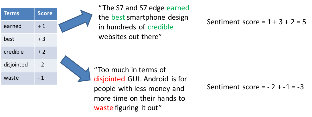
There are many different methods and approaches to sentiment analysis. Here we cover only the most basic approaches to sentiment analysis. However, nothing prevents you from adopting a more sophisticated approach using NLP and other tools. The following diagram illustrates the approach taken in this how-to.

twitter-sentiment-spark-20

The sentiment figures will be a rough gauge of how positive or negative the tweets are about the subject. There are several key simplifications taken in the interest of time that you may want to explore further to improve the accuracy of sentiment analysis:

  • Retweets are considered as “having the same sentiment” – obviously, this may not be true but it would simplify the way tweets are processed
  • The presence of the subject will “take on” the sentiment of the tweet. This means that if Samsung S7 is mentioned in the tweet, the sentiment of the tweet is attributed to “Samsung S7”. Obviously, in order to be more accurate, we would need to do entity-name resolution, sentence parsing and aspect based sentiment analysis. But to stay on focus on this tutorial, we will not be covering these topics (perhaps in a subsequent post)
  • Sarcasm and word inflexions are not taken into account and may lead to the following incorrect sentiment scoring as shown below:

twitter sentiment spark-25.png


Nonetheless, this is not to say we cannot do sentiment analysis – but rather to highlight on the difficulties in getting the right sentiment – which will not be address in this tutorial.


Introduction to PySpark

It has been several years since the introduction of Hadoop and Spark and for a while there was some confusion in their roles as Big Data engineering tools. However, in recent times, their role as supporting components rather than competing products has been widely accepted. Nontheless, I am sharing some definitions of what Spark is from multiple sources which I found useful to highlight the key capabilities / purposes of Spark:

  • Apache Spark is a lightning-fast cluster computing technology, designed for fast computation. It is based on Hadoop MapReduce and it extends the MapReduce model to efficiently use it for more types of computations, which includes interactive queries and stream processing. The main feature of Spark is its in-memory cluster computing that increases the processing speed of an application. (https://www.tutorialspoint.com/apache_spark/apache_spark_introduction.htm)

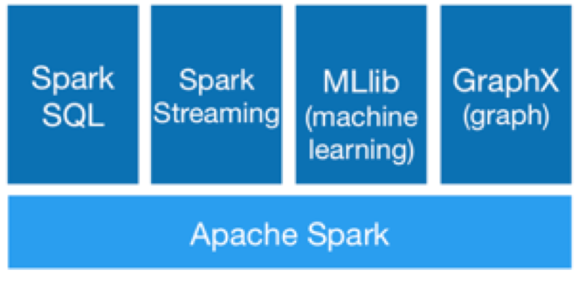
The components of Spark are as shown below and we will be mainly using SparkSQL and PySpark.

twitter-sentiment-spark-21

To find out more about Spark you can refer to the following: http://spark.apache.org/docs/latest/index.html

PySpark 

Spark is written in Scala and Spark applications during compilation are translated into Java bytecode for execution by the JVM. However, the open source community has developed a toolkit to allow users to write programs in Python (which will still compile down to Java bytecode) called PySpark.

I recommend that you read through the following to understand what you will be coding in the following sections


Twitter Message and Candidate Attribution

To simplify this tutorial, how we determine if a tweet is to be attributed to a candidate / subject is by referencing the candidate / subjects handle. For example:

  • Tweet #2
    • @realDonaldTrump wining, lying, Donald Trump, does not make a president
  • Tweet #3
    • @Colonel_Ted: Even if @realDonaldTrump picked @tedcruz (MY fave) for VP I can NEVER in good conscience vote for this megalomaniac. https…

In the tweets above, we will identify the various named entities by their handles @realDonaldTrump, @Colonel_Ted, @tedcruz. Hence the sentiment for the tweet will be attributed to the entities referenced by their Twitter handles.

So in the example above, the sentiment for tweets #1 and #2 will be attributed to Donald Trump, while tweet #3 will be attributed to Donald Trump AND Ted Cruz

As we are taking a very simplistic approach to sentiment attribution, we can use this approach. However, for a more accurate sentiment analysis, I would strongly recommend to do NLP, ENR and aspect based sentiment analysis.

Sentiment Analysis Code

The following steps outline the approach in determining the sentiments of the tweets.

Step 1: Create a simple mapping to label the tweet name. Because different candidates will be referenced in the tweet differently we would need to map each candidate name to the different names they are referred by.

Step 2: Create a dictionary of sentiment words and its associated scores. This will be used to calculate the overall sentiment score of the tweet.

Step 3: For each tweet, calculate the sentiment score and total the score for each candidate

Copy the following code into a file “SentimentAnalysis.py” and save it on the ./SentimentAnalysis folder (refer to Tutorial 1 for the folder location)

#!/usr/bin/env python
#
# Licensed to the Apache Software Foundation (ASF) under one or more
# contributor license agreements.  See the NOTICE file distributed with
# this work for additional information regarding copyright ownership.
# The ASF licenses this file to You under the Apache License, Version 2.0
# (the "License"); you may not use this file except in compliance with
# the License.  You may obtain a copy of the License at
#
#    http://www.apache.org/licenses/LICENSE-2.0
#
# Unless required by applicable law or agreed to in writing, software
# distributed under the License is distributed on an "AS IS" BASIS,
# WITHOUT WARRANTIES OR CONDITIONS OF ANY KIND, either express or implied.
# See the License for the specific language governing permissions and
# limitations under the License.
#
# Code to score tweets using AFINN and to generate a set of sentiment score for each person mentioned.
#   usage: ./bin/pyspark SentimentAnalysis.py
#

"""SentimentAnalysis.py"""

import math
import re
import sys

from StringIO import StringIO
from datetime import datetime
from collections import namedtuple
from operator import add, itemgetter

# Note - SparkContext available as sc, HiveContext available as sqlCtx.
from pyspark import SparkContext
from pyspark import HiveContext
from pyspark.streaming import StreamingContext

sc = SparkContext(appName="PythonSentimentAnalysis")
sqlCtx = HiveContext(sc)

# Read in the word-sentiment list and create a static RDD from it
filenameAFINN = "/home/training/TwitterSentimentAnalysis/AFINN/AFINN-111.txt"

# map applies the lambda function (create a tuple of word and sentiment score) to every item of iterable
# within [ ] and returns a list of results. The dictionary is used here to be able to quickly lookup the
# sentiment score based on the key value
afinn = dict(map(lambda (w, s): (w, int(s)), [ ws.strip().split('\t') for ws in open(filenameAFINN) ]))

# Read in the candidate mapping list and create a static dictionary from it
filenameCandidate = "file:///home/training/TwitterSentimentAnalysis/Candidates/Candidate Mapping.txt"

# map applies the lambda function
candidates = sc.textFile(filenameCandidate).map(lambda x: (x.strip().split(",")[0],x.strip().split(","))) \
				  	   .flatMapValues(lambda x:x).map(lambda y: (y[1],y[0])).distinct()

# word splitter pattern
pattern_split = re.compile(r"\W+")

# use sqlCtx to query the HIVE table
tweets = sqlCtx.sql("select id, text, entities.user_mentions.name from incremental_tweets")

#this python function will calculate the sentiment score of the entire tweet
def sentiment(text):
 words = pattern_split.split(text.lower())
 sentiments = map(lambda word: afinn.get(word, 0), words)
 if sentiments:
  sentiment = float(sum(sentiments))/math.sqrt(len(sentiments))
  #sentiment = float(sum(sentiments))
 else:
  sentiment = 0
 return sentiment

sentimentTuple = tweets.rdd.map(lambda r: [r.id, r.text, r.name]) \
			   .map(lambda r: [sentiment(r[1]),r[2]]) \
			   .flatMapValues(lambda x: x) \
			   .map(lambda y: (y[1],y[0])) \
			   .reduceByKey(lambda x, y: x+y) \
			   .sortByKey(ascending=True)

scoreDF = sentimentTuple.join(candidates) \
			.map(lambda (x,y): (y[1],y[0])) \
			.reduceByKey(lambda a,b: a+b) \
			.toDF()

scoreRenameDF = scoreDF.withColumnRenamed("_1","Candidate").withColumnRenamed("_2","Score")

sqlCtx.registerDataFrameAsTable(scoreRenameDF, "SCORE_TEMP")

sqlCtx.sql("INSERT OVERWRITE TABLE candidate_score SELECT Candidate, Score FROM SCORE_TEMP")

The statements above are self-explanatory but I will take some time to discuss the key statements in this entire script as follows:

sentimentTuple = tweets.rdd.map(lambda r: [r.id, r.text, r.name]) \
			   .map(lambda r: [sentiment(r[1]),r[2]]) \
			   .flatMapValues(lambda x: x) \
			   .map(lambda y: (y[1],y[0])) \
			   .reduceByKey(lambda x, y: x+y) \
			   .sortByKey(ascending=True)

scoreDF = sentimentTuple.join(candidates) \
			.map(lambda (x,y): (y[1],y[0])) \
			.reduceByKey(lambda a,b: a+b) \
			.toDF()

The following describes what each line in the above statement is doing.

sentimentTuple = tweets.rdd.map(lambda r: [r.id, r.text, r.name])

The result set from the query of tweets is referenced as a Resilient Data Set (.rdd) and then the lambda function is applied to all the rows in the RDD using the map method. The “map” method can be thought of as the “map” in “map-reduce”.

Note that the lambda function takes in a row of the RDD (in parameter r) and we create a list of 3-tuples (r.id, r.text, r.name)

[724232069421768704, u”@LewisHShupe I’m tired of being penalized for not having #Obamacare because I can’t afford it/ @BarackObama is a #POS #terrorist #TrumpTrain”, [u’Lewis Shupe’, u’Barack Obama’]]

r.id r.text r.name
724232069421768704 “@LewisHShupe I’m tired of being penalized for not having #Obamacare because I can’t afford it/ @BarackObama is a #POS #terrorist #TrumpTrain Lewis Shupe, Barack Obama
.map(lambda r: [sentiment(r[1]),r[2]]) \

With the list of 3-tuples, we again apply the lambda function on each row (now a 3-tuple) that calls the sentiment function earlier defined and returns a 2-tuple – sentiment score and r.text (r[2])

[1.0425720702853738, [u'Hillary Clinton']],
[-0.47140452079103173, [u'RTina']],
[-0.4082482904638631, [u'Lewis Shupe', u'Barack Obama']],
[-1.3093073414159544, [u'CJLB', u'Ted Cruz', u'Jim Hoft']]
sentiment(r[1]) r[2]
1.0425720702853738 Hillary Clinton
-0.47140452079103173 RTina
-0.4082482904638631 Lewis Shupe, Barack Obama
-1.3093073414159544 CJLB, Ted Cruz, Jim Hoft
.flatMapValues(lambda x: x) \

With the 2-tuple dataset, we apply a flatMapValues function to flatten out the structure within r[2]. This will make it easier to process in the subsequent steps

(1.0425720702853738, u'Hillary Clinton'), (-0.47140452079103173, u'RTina'), (0.0, u'Halli Casser-Jayne'), (0.0, u'Yvonne Slee '), (0.0, u'Raymond W Clarke'), (-1.3093073414159544, u'CJLB'), (-1.3093073414159544, u'Ted Cruz'), (-1.3093073414159544, u'Jim Hoft')
sentiment(r[1]) r[2]
1.0425720702853738 Hillary Clinton
-0.47140452079103173 RTina
-0.4082482904638631 Lewis Shupe
-0.4082482904638631 Barack Obama
-1.3093073414159544 CJLB
-1.3093073414159544 Ted Cruz
-1.3093073414159544 Jim Hoft
.map(lambda y: (y[1],y[0])) \

This is a simple step to swap the fields so that the first column is the name and the second is the sentiment score

y[1] y[0]
Hillary Clinton 1.0425720702853738
RTina -0.47140452079103173
Lewis Shupe -0.4082482904638631
Barack Obama -0.4082482904638631
CJLB -1.3093073414159544
Ted Cruz -1.3093073414159544
Jim Hoft -1.3093073414159544
.reduceByKey(lambda x, y: x+y) \

The reduceByKey is a function where the values of the 2-tuples are added together. By default the first column in the data set will be the key – hence this statement will add all the y[0] having the same key value in y[1]. The result of summing each name found in the entire set of tweets is as shown below (first 6 only, not sorted in any order)

(u'Ava Guthrie', -1.6329931618554523)
(u'K Kelly', 0.0)
(u'AUBURN FAN 4 RUBIO', -0.6255432421712244)
(u'Royal Jordanian', 0.47140452079103173)
(u'JOEY MANNARINO', 6.4236405483757295)
(u'Jimmy Kimmel', -0.75)
.sortByKey(ascending=True)

Finally the sortByKey method will sort the 2-tuple RDD in ascending order by name. In the sample extract below, the first 10 2-tuples sorted by name is as shown below:

(u'#$@%&+?', 0.47140452079103173)
(u'#1 Road Warrior Fan', 0.0)
(u'#4thewin', 0.8121063121025829)
(u'#Alwaystrump', -1.4278802916547295)
(u'#AngryMajorityNY', 1.6417736995057388)
(u'#BERNIEFACTS', 0.20062843367526345)
(u'#BLACKS FOR TRUMP!!!', 0.0)
(u'#BargainingChip', 0.4364357804719848)
(u'#BlackLivesMatter-LA', 0.0)
(u'#Chemtrails', -0.5345224838248488)
scoreDF = sentimentTuple.join(candidates) \
			.map(lambda (x,y): (y[1],y[0])) \
			.reduceByKey(lambda a,b: a+b) \
			.toDF()

The last step would be to do a left join with the candidates dataframe so that only the 2-tuple sentiment scores for the candidate names we are interested in will be returned and we then sum them up by the mapped name before returning the final sentiment score.

Row(_1=u’Hillary Clinton’, _2=2.508604778151232)
Row(_1=u’Donald Trump’, _2=76.03149029470246)
Row(_1=u’Ted Cruz’, _2=162.63942375987867)
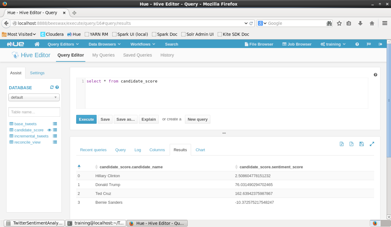
Row(_1=u’Bernie Sanders’, _2=-10.372575217548247)

Copy Supporting Files

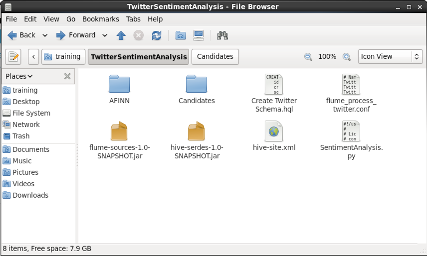
Ensure that the following are in the same folder as the “SentimentAnalysis.py” file.

  • AFINN folder with AFINN-96.txt, AFINN-111.txt and AFINN-README.txt
  • Candidates folder with Candidate Mapping.txt
  • hive-site.xml

The folder should look like the one below:

twitter-sentiment-spark-22

Running the PySpark Script

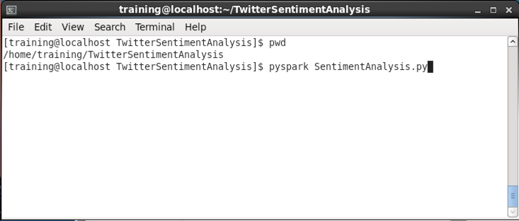
Before running the SentimentAnalysis.py script, ensure that you are at the /TwitterAnalysis/ folder.

twitter-sentiment-spark-23

You should eventually see the Spark job complete and you can then navigate back to the Hive Editor and execute the query:

select * from candidate_score to view the results of the Spark job.

twitter-sentiment-spark-24

Finally, you can then use your favorite visualization tool to plot the results.


Possible Errors Encountered

During the execution of the Python script you may encounter the following error:

Py4JJavaError: An error occurred while calling o44.sql.
: java.lang.RuntimeException: java.lang.RuntimeException: Unable to instantiate org.apache.hadoop.hive.ql.metadata.SessionHiveMetaStoreClient
......
Caused by: java.lang.RuntimeException: Unable to instantiate org.apache.hadoop.hive.ql.metadata.SessionHiveMetaStoreClient
……
Caused by: javax.jdo.JDOFatalInternalException: Error creating transactional connection factory
NestedThrowables:
java.lang.reflect.InvocationTargetException

This could be caused by a missing hive-site.xml file in the /TwitterAnalysis/ folder or when running the script you are not running from /TwitterAnalysis/.

Resolution:


Final Words

I hope you have found the 3-part tutorial helpful in understanding Hadoop, Hive, Flume, Spark and PySpark. Here are some of my afterthoughts


Observations

  • Cloudera VM is preloaded with older versions of Spark and HIVE
  • Further configuration required to ensure SparkSQL works on HIVE files. Additional libraries and configuration filed required
  • Flume configuration is a non-trival activity and needs to find the correct libraries for Twitter integration (apache vs cloudera)


Further Architecture Improvements

  • HIVE on HDFS performance can be improved though partitioning by date – this will allow us to query the sentiment and compare across dates easier.
  • Consider using Impala (however needs to explore the configuration setup required, libraries, config files)
  • Move to Spark Streaming directly ingesting from HIVE to stream processing of the sentiment scoring (currently using batch processing)
  • HIVE supports ACID since 0.13 however, there is performance impact due to transaction management. Hence need to put in place workflow (e.g. Oozie) to process inbound messages in staging and move processed messages to processed table instead of transactional updates.


Further Analytic Improvements

  • Use StandfordNLP and Python NLTP to do entity based sentiment analysis. This would provide a more accuract sentiment scoring for each candidate
  • Plot and track sentiment scoring across time period to understand how each candidate is being view from the social media space

Simple Twitter Sentiment Analytics Using Apache Flume and Spark – Part 2

In my last post, on the same topic above, I outlined the steps, possible issues and how to overcome them when setting up Hive tables, Flume and getting to query the data through Hive.

I realized that there wasn’t any explanation on the structure of the Flume configuration file. Understanding how the Flume configuration file is structured enabled me to quickly configure and understand the basics of setting up Flume and I think this would be useful to anyone who wants to start working with Flume.

As per my experience on new tools (at least new to me), the documentation took me some time to understand and digest and I had to trawl through the web for examples for me to learn.

I will give a quick and brief description of the Flume configuration file so that at the least it will make sense for you when you work on this tutorial / exercise, this will be done section by section as follows.

Lets start!

Flume Sources, Channels and Sinks

A typical way to view how data will be ingested is to think in terms of Sources, Channels and Sinks. Sources define well sources of data. Sinks define the target by which the data will be persisted to. Channels refer to the way the data will be transferred between sources and sinks.

The first thing to do is to define the Sources, Channels and Sinks for a Flume connection.

# Naming the components on the current agent.
TwitterAgent.sources = Twitter
TwitterAgent.channels = MemChannel
TwitterAgent.sinks = HDFS

Typically, the above section details the source, channel and sink for Flume to operate on. Note that Flume can handle multiple sources, channels and sinks within a single configuration file. However, for this exercise / tutorial we will keep it simple with only 1 source, 1 channel and 1 sink.

Here, the string “TwitterAgent” refers to the name of the Flume agent that the properties of “sources”, “channels” and “sinks” belong to.

In essence, by specifying “TwitterAgent” as the string before “sources”, we are configuring the sources property of the Flume agent named “TwitterAgent”. This is important as we will refer to this agent name when running Flume.

Here we have specified the sources to be “Twitter”, using “MemChannel” as the channel and “HDFS” as the sink. The reason why I have put them in quotes will be revealed later. You could have also used any other string – e.g. “Twtr”, “M1”, “S1” etc … to refer to the sources, channels and sinks, but I chose this naming convention to ensure readability.

Generally, naming the components in Flume takes on the following convention:

<agent_name>.sources = <source_name>
<agent_name>.channels = <channel_name>
<agent_name>.sinks = <sink_name>


Describing the Source

A source will have a list of properties. The property “type” is common to every source, and it is used to specify the type of the source we are using. Examples of source types are: HTTP, Twitter, UDP etc.

# Describing/Configuring the source
TwitterAgent.sources.Twitter.type = com.cloudera.flume.source.TwitterSource
TwitterAgent.sources.Twitter.consumerKey = <consumer key>
TwitterAgent.sources.Twitter.consumerSecret = <consumer secret>
TwitterAgent.sources.Twitter.accessToken = <access token>
TwitterAgent.sources.Twitter.accessTokenSecret = <access token secret>
TwitterAgent.sources.Twitter.keywords = @realDonaldTrump, @HillaryClinton, @SenSanders, @BernieSanders, @tedcruz, #election2016, #hillaryclinton, #hillary, #hillary2016, #Hillary2016, #donaldtrump, #trump, #dumptrump, #pooptrump, #turdtrump, #sanders, #tedcruz, #feelthebern, #dontfeelthebern, #bernie2016, #trump2016, #whybother2016, #trumptrain, #notrump, #whichhillary, #voteforbernie, #sandersonly, #americafortrump, #berniecrats, #berniestrong, #berniesanders2016, #imwithher, #killary, #stepdownhillary, #stophillary, #vote2016

Some sources such as Twitter may require specific Java libraries such as:

com.cloudera.flume.source.TwitterSource
com.apache.flume.source.TwitterSource

You will need to find out if your desired source is supported and if there are any implementation specific libraries required.

Other than the property “type”, different sources may have other required properties of a particular source. For example, if you use the Twitter source as described above, you will be required to include the  consumerKey, consumerSecret, accessToken, accessTokenSecret properties. If you had chosen HTTP another different set of properties would then be required to be entered.

You will need to find out for each source type, what are the specific required properties you need to provide in the configuration. This will probably be the most challenging thing during the creation of the Flume config script.

In the above example, the keywords to filter the tweets are defined in the property “keywords”. This means that Flume will capture tweets with any of the above listed keywords.

Specifying the source properties in Flume takes on the following convention:

<agent_name>.sources.<source_name>.type = <value>
<agent_name>.sources.<source_name>.<property2> = <value>
<agent_name>.sources.<source_name>.<property3> = <value>


Describing the Sink

Similar to the source, each sink (in the case of multiple sinks) will have a separate list of properties. The property “type” is common to every source, and it is used to specify the type of the source we are using. Other than the property “type”, different sinks may have other required properties of a particular sink, as shown below.

# Describing/Configuring the sink
TwitterAgent.sinks.HDFS.type = hdfs
TwitterAgent.sinks.HDFS.hdfs.path = /twitteranalytics/incremental
TwitterAgent.sinks.HDFS.hdfs.fileType = DataStream
TwitterAgent.sinks.HDFS.hdfs.writeFormat = Text
TwitterAgent.sinks.HDFS.hdfs.filePrefix = twitter-
TwitterAgent.sinks.HDFS.hdfs.rollInterval = 0
TwitterAgent.sinks.HDFS.hdfs.rollSize = 524288
TwitterAgent.sinks.HDFS.hdfs.rollCount = 0
TwitterAgent.sinks.HDFS.hdfs.idleTimeout = 0
TwitterAgent.sinks.HDFS.hdfs.batchSize = 100
TwitterAgent.sinks.HDFS.hdfs.threadsPoolSize = 2
TwitterAgent.sinks.HDFS.hdfs.round = true
TwitterAgent.sinks.HDFS.hdfs.roundUnit = hour

In the example above, the sink type is “hdfs” and the properties belonging to the sink type HDFS are shown above. You can refer to this website for the list of properties and their definitions: http://hadooptutorial.info/flume-data-collection-into-hdfs/

Specifying the sink properties in Flume takes on the following convention:

<agent_name>.sinks.<source_name>.type = <value>
<agent_name>.sinks.<source_name>.<property2> = <value>
<agent_name>.sinks.<source_name>.<property3> = <value>

Note that for HDFS, the property format is hdfs.<property>


Describing the Channel

The channel configuration is similar to that of sources and sinks and is as shown below:

# Describing/Configuring the channel
TwitterAgent.channels.MemChannel.type = memory
TwitterAgent.channels.MemChannel.capacity = 10000
TwitterAgent.channels.MemChannel.transactionCapacity = 100

You can refer to this website for the list of properties and their definitions: http://archive.cloudera.com/cdh4/cdh/4/flume-ng/FlumeUserGuide.html#flume-channels


Bindings

Finally, to connect the source, channel and sinks together the following needs to be declared in the configuration file. The following configuration specifies that the Twitter source and HDFS sink are both using the same channel “MemChannel”. This effectively binds the source and the sink.

# Binding the source and sink to the channel
TwitterAgent.sources.Twitter.channels = MemChannel
TwitterAgent.sinks.HDFS.channel = MemChannel


Starting Flume Agent

When starting Flume, you will now specify the specific agent and its relevant configuration to be started as follows:

flume-ng agent -f flume_process_twitter.conf Dflume.root.logger=DEBUG,console -n TwitterAgent

As you will notice, the –name, -n <name> command line parameter specifies the specific agent to execute. Since in this case, the agent name in the configuration file is TwitterAgent, hence all the configuration settings beginning with TwitterAgent will be applied.

Note that this allows us to specify multiple different agents within the same single configuration file.

That’s it!

We have covered a brief overview and walkthrough on configuring Flume. I hope this will help you understand the structure of the Flume configuration file and how to set it up for your next big data project!

Here are links to some of the websites and how-tos which I have found helpful in understanding how to setup Flume.


In the next post, I will go through in detail how to use Spark to execute the sentiment analysis.


Simple Twitter Sentiment Analytics Using Apache Flume and Spark – Part 1

Its been some time since my last post but am excited to be sharing about my learnings and adventures with Big Data and Data Analytics.

Recently I had the opportunity to do some simple Twitter sentiment analytics using a combination of HDFS, Hive, Flume and Spark and wanted to share how it was done.

While many other blogs do cover a great deal on how to do the above, I wanted to also share some of the errors I encountered and how to resolve them, hopefully saving you time from searching the web and trying all kinds of solutions.

You can download the source files in this how-to for your easy reference here. Remember to save them in your local folders on the Cloudera VM.

Ready? Lets start!

Step 1: Getting Cloudera Hadoop CDH5.4.3a ready

We begin by first setting up and installing Cloudera Hadoop CDH5.4.3a. Ensure that you run any preconfigured scripts to ensure that Flume, Spark, Python, HDFS, Hive, Hue, Impala, Zookeeper, Kafka, Slor are setup and configured.

For this exercise, I am using a pre-configured Hadoop stack setup from Cloudera. If you have another distribution, you should still be able to run this how-to. However the issues encountered in this tutorial may differ for different distributions.

The version of HDFS used in this tutorial is Hadoop 2.6.0-cdh5.4.3, however the instructions and steps here should be application for any subsequent versions.

This tutorial assumes that you are familiar with hdfs commands. If not, you can refer to this link here.

Step 2: Ensuring that Hive is working

In the VM environment, ensure that Hive2 server is started. Run the following command to start Hive2 server.

sudo service hive-server2 start

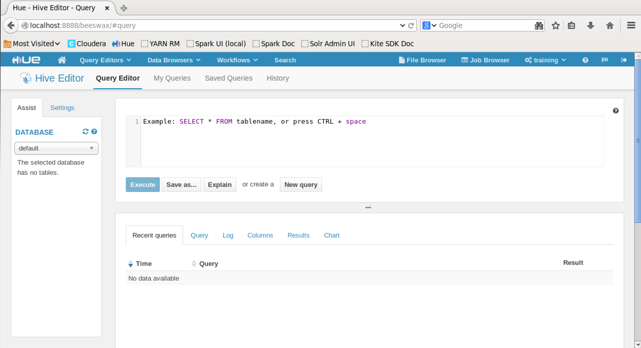
Once the server is successfully started, login to Hue and click on Query Editors > Hive to view the Query Editor page.

twitter sentiment spark-1

Step 3: Create HDFS Folder

In this project, we will access the Twitter API to download the tweets and the downloaded files will be saved onto HDFS and access through Hive tables. First, create the following directory structure in HDFS.

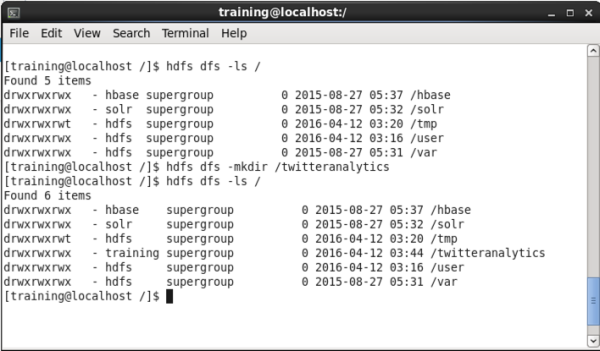
twitter sentiment spark-2

Run the above command instructs HDFS to create a folder “twitteranalytics” in the top level of the HDFS directory. A standard directory structure is used in HDFS that is similar to a typical file system in Unix. However, one of the key differences is that there is no concept of a current directory within HDFS. Hence HDFS files are referred to by their fully qualified name which is a parameter of many of the elements of the interaction between the Client and the other elements of the HDFS architecture. See this site for more details on the HDFS architecture.

If you do an “ls” command in HDFS you should see the directory you have just created as shown below.

twitter sentiment spark-11

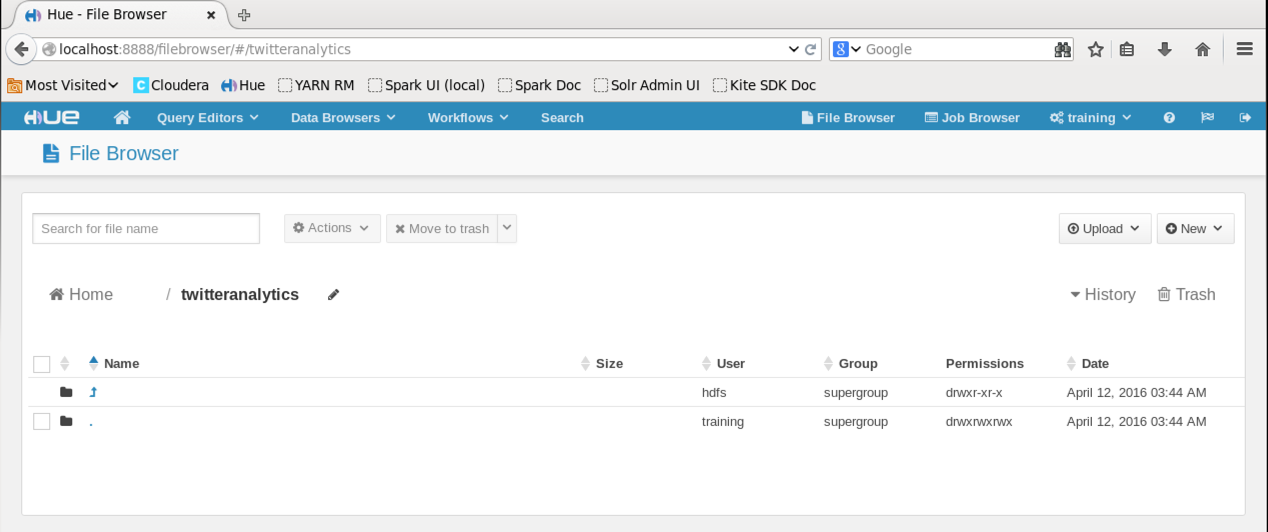
Use the File Browser in Hue to view the folder you have just created.

twitter sentiment spark-3

Once done, you can now start to create the table schema from the Hive script – “Create Twitter Schema.hql” (Note: This can be found in the Github repository)

Step 4: Create Hive Tables

Before you can run the Hive script to create the tables, you must ensure that the JSON serdes (Serializer / Deseralizer) library is available otherwise you will get the following error:

“FAILED: Execution Error, return code 1 from org.apache.hadoop.hive.ql.exec.DDLTask. Cannot validate serde: com.cloudera.hive.serde.JSONSerDe”

Run the following command to copy the hive-serdes-1.0-SNAPSHOT.jar file to the Hive lib directory.

sudo cp hive-serdes-1.0-SNAPSHOT.jar /usr/lib/hive/lib

Next restart the Hive2 server with the following commands

sudo service hive-server2 stop
sudo service hive-server2 start

Run the Hive script in the command line to create the tables as follows

hive -f Create\ Twitter\ Schema.hql

The result should be as shown below and this confirms that the script has been successfully executed and the tables created.

twitter sentiment spark-4

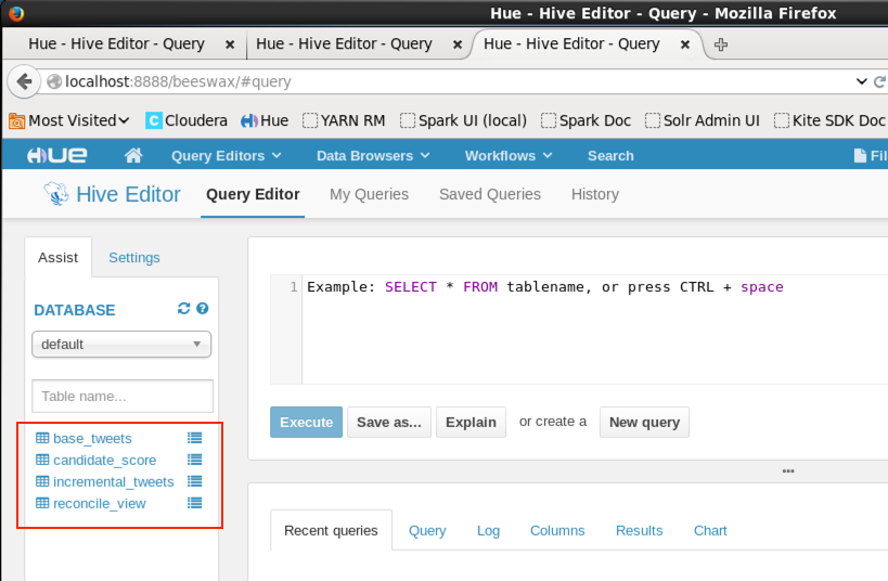
Go back to Hue > Query Editors > Hive and refresh the database list. You should now see the following tables created against the default database. Note that one of the tables is actually a VIEW.

twitter sentiment spark-5

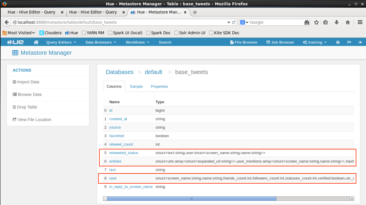
Congratulations! You have successfully created Hive tables on HDFS. Lets take a look at the tables in detail. In Hue, navigate to Data Browsers > Metastore Tables and click on base_tweets table.

twitter sentiment spark-6

The table structure can be viewed and you would notice that several columns have a struct as their definition. This is how a JSON file will be represented in Hive and that’s the reason why you would need a JSON SerDes library, to interprete and translate the JSON structure into a “query-able” schema.

For more information about JSON, Hive and HDFS, please click on the links below:

https://cwiki.apache.org/confluence/display/Hive/Json+SerD
http://stackoverflow.com/questions/14705858/using-json-serde-in-hive-tables
http://stackoverflow.com/questions/11479247/how-do-you-make-a-hive-table-out-of-json-data

The reason we are using JSON structure is because the Twitter feed is in the form of a JSON file. For more information on the Twitter JSON structure please refer to Twitter developer documentation here – https://dev.twitter.com/streaming/overview

Step 5: Configure Flume

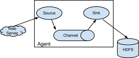
The next step would be to create the Flume configuration file to connect to Twitter (source) and persist the JSON files on HDFS (sink). Conceptually the flow is as illustrated from the Apache Flume website:

devguide_image00

Create a local folder for this project and name it “TwitterSentimentAnalysis”. This folder can be in your home directory. Navigate to the folder and create a Flume configuration file as follows:

vi flume_process_twitter.conf

twitter sentiment spark-7

Copy and paste the following code and save the file.

# Naming the components on the current agent.
TwitterAgent.sources = Twitter
TwitterAgent.channels = MemChannel
TwitterAgent.sinks = HDFS

# Describing/Configuring the source
TwitterAgent.sources.Twitter.type = com.cloudera.flume.source.TwitterSource
TwitterAgent.sources.Twitter.consumerKey = <enter your consumer key>
TwitterAgent.sources.Twitter.consumerSecret = <enter your consumer secret>
TwitterAgent.sources.Twitter.accessToken = <enter your access token>
TwitterAgent.sources.Twitter.accessTokenSecret = <enter your access token secret>
TwitterAgent.sources.Twitter.keywords = @realDonaldTrump, @HillaryClinton, @SenSanders, @BernieSanders, @tedcruz, #election2016, #hillaryclinton, #hillary, #hillary2016, #Hillary2016, #donaldtrump, #trump, #dumptrump, #pooptrump, #turdtrump, #sanders, #tedcruz, #feelthebern, #dontfeelthebern, #bernie2016, #trump2016, #whybother2016, #trumptrain, #notrump, #whichhillary, #voteforbernie, #sandersonly, #americafortrump, #berniecrats, #berniestrong, #berniesanders2016, #imwithher, #killary, #stepdownhillary, #stophillary, #vote2016

# Describing/Configuring the sink
TwitterAgent.sinks.HDFS.type = hdfs
TwitterAgent.sinks.HDFS.hdfs.path = /twitteranalytics/incremental
TwitterAgent.sinks.HDFS.hdfs.fileType = DataStream
TwitterAgent.sinks.HDFS.hdfs.writeFormat = Text

TwitterAgent.sinks.HDFS.hdfs.filePrefix = twitter-
TwitterAgent.sinks.HDFS.hdfs.rollInterval = 0
TwitterAgent.sinks.HDFS.hdfs.rollSize = 524288
TwitterAgent.sinks.HDFS.hdfs.rollCount = 0
TwitterAgent.sinks.HDFS.hdfs.idleTimeout = 0
TwitterAgent.sinks.HDFS.hdfs.batchSize = 100
TwitterAgent.sinks.HDFS.hdfs.threadsPoolSize = 2
TwitterAgent.sinks.HDFS.hdfs.round = true
TwitterAgent.sinks.HDFS.hdfs.roundUnit = hour

# Describing/Configuring the channel
TwitterAgent.channels.MemChannel.type = memory
TwitterAgent.channels.MemChannel.capacity = 10000
TwitterAgent.channels.MemChannel.transactionCapacity = 100

# Binding the source and sink to the channel
TwitterAgent.sources.Twitter.channels = MemChannel
TwitterAgent.sinks.HDFS.channel = MemChannel

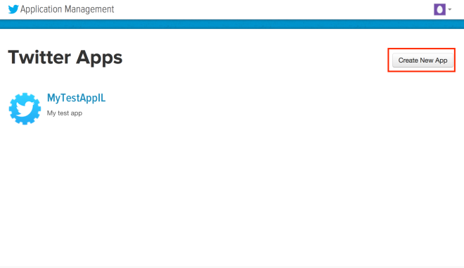
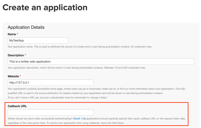
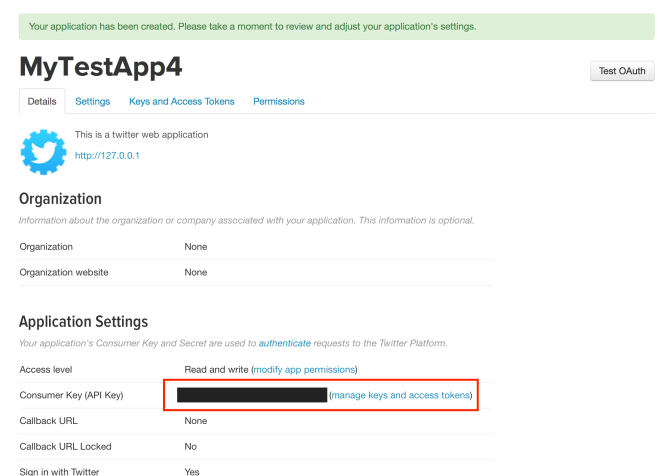
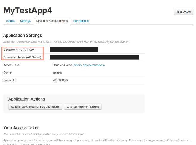
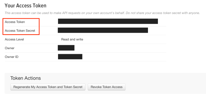
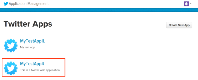
Please note that you would need to have a Twitter Dev account and create a Twitter App so as to get your consumerKey, consumerSecret, accessToken and accessTokenSecret.

Once the config file has been successfully created, enter the following Flume command to start the Flume agent.

flume-ng agent -f flume_process_twitter.conf Dflume.root.logger=DEBUG,console -n TwitterAgent

When trying to execute the flume agent, here are some possible errors you may encounter and how to resolve them:

  • Unable to load source type: com.cloudera.flume.source.TwitterSource
“ERROR node.PollingPropertiesFileConfigurationProvider: Failed to load configuration data. Exception follows.
org.apache.flume.FlumeException: Unable to load source type: com.cloudera.flume.source.TwitterSource, class: com.cloudera.flume.source.TwitterSource”

Ensure that “flume-sources-1.0-SNAPSHOT.jar” is copied to the following directories:

/var/lib/flume-ng/plugins.d/twitter-streaming/lib
/usr/lib/flume-ng/plugins.d/twitter-streaming/lib

If the specific folders are not created, please create them as per structure above

Refer to the StackOverflow threads here for more information: http://stackoverflow.com/questions/19189979/cannot-run-flume-because-of-jar-conflict

  • java.lang.NoSuchMethodError:twitter4j.FilterQuery.setIncludeEntities(Z)Ltwitter4j/FilterQuery
“ERROR lifecycle.LifecycleSupervisor: Unable to start EventDrivenSourceRunner: { source:com.cloudera.flume.source.TwitterSource{name:Twitter,state:IDLE} } - Exception follows.
java.lang.NoSuchMethodError: twitter4j.FilterQuery.setIncludeEntities(Z)Ltwitter4j/FilterQuery;”

This is probably because of a conflict in the twitter4j-stream libraries. You would need to rename the following jar files: twitter4j-stream-3.0.3.jartwitter4j-core-3.0.3.jar and twitter4j-media-support-3.0.3.jar

sudo mv /usr/lib/flume-ng/lib/twitter4j-stream-3.0.3.jar /usr/lib/flume-ng/lib/twitter4j-stream-3.0.3.jarx
sudo mv /usr/lib/flume-ng/lib/twitter4j-core-3.0.3.jar /usr/lib/flume-ng/lib/twitter4j-core-3.0.3.jarx
sudo mv /usr/lib/flume-ng/lib/twitter4j-media-support-3.0.3.jar /usr/lib/flume-ng/lib/twitter4j-media-support-3.0.3.jarx

Refer to the StackOverflow threads here for more information: http://stackoverflow.com/questions/24322028/cdh-twitter-example-java-error

Step 6: Monitoring Flume Agent and Querying Tweets

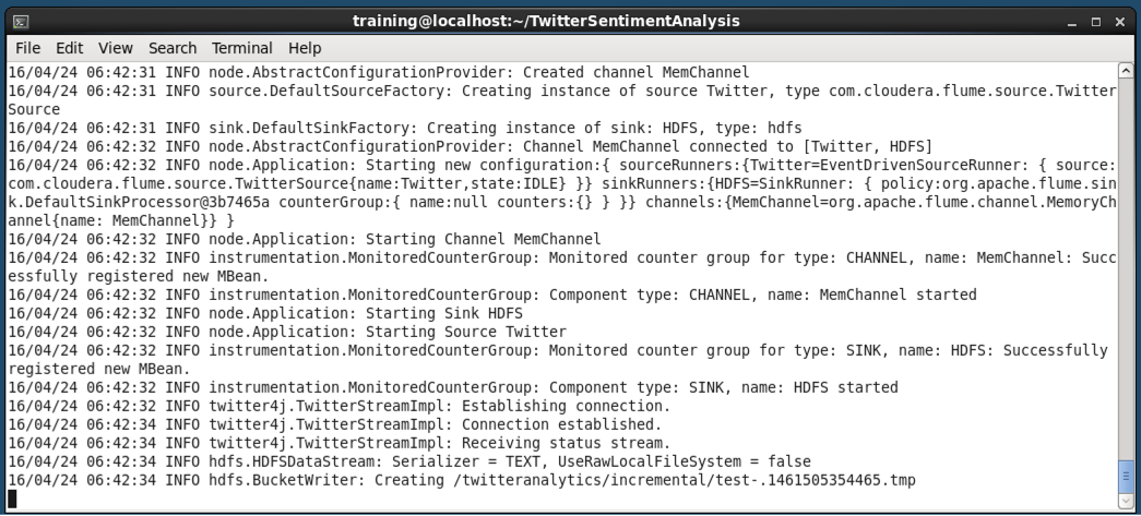
Once the Flume agent is successfully started, you would be able to see the console logs as shown below. The console will refresh as the tweets are being received by Flume and persisted in HDFS.

twitter sentiment spark-8

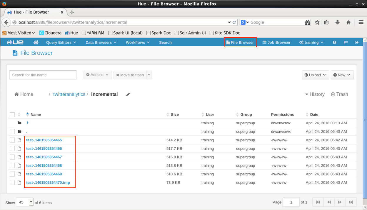
You can verify that Flume is reading from Twitter and creating the JSON files by navigating to Hue > File Browser > /twitteranalytics/incremental as shown below.

twitter sentiment spark-9

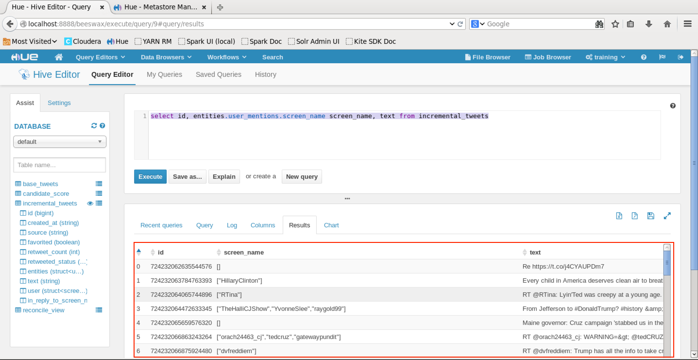
To verify that the tweet data can be viewed through Hive, you can navigate in Hue to Query Editors > Hive and on the query editor enter the following SQL

select id, entities.user_mentions.screen_name screen_name, text from incremental_tweets

The above SQL will query the Hive table incremental_tweets for the ID, screen_name field that is part of the user_mentions structure and the tweet text. You should get the following result:

twitter sentiment spark-10

The result is presented just like any SQL result set – with the exception of columns where the “[]” represent the JSON substructure.

That’s it! Well done!

You have successfully used Flume to receive streaming tweets, created Hive tables to store the data on HDFS and used SQL to retrieve the stored information.

Hope you have found this how-to useful! In the next post, we will create a Spark job in Python to determine the sentiment of the tweets.

You can download the Flume configuration and source files for your easy reference here.

rJava load error in RStudio/R after upgrading to OS X El Capitan

It appears that every time there is an upgrade of OS X, rJava will break. I had this experience with Yosemite and now El Capitan as well.

After many hours of figuring out what went wrong, it came down to the “Rootless” security feature in OS X.

Previously, I was able to run rJava on Yosemite following the instructions found on this forum post on Stack Overflow here. When you eventually run the command:

sudo ln -f -s $(/usr/libexec/java_home)/jre/lib/server/libjvm.dylib /usr/lib

the following error will appear:

rJava Issues-1

This is because the “Rootless” security feature in OS X El Capitan will no longer allow us to write to /usr/lib. Instead, you should be running the command

sudo ln -f -s $(/usr/libexec/java_home)/jre/lib/server/libjvm.dylib /usr/local/lib

Note that the path should now be /usr/local/lib. This will create the symbolic link that will allow R/RStudio to load the ibjvm.dylib and enable rJava to run properly.

Hope this will be helpful to those who are struggling with rJava on El Capitan!

Here are some other links about the Rootless security feature in OSX (courtesy of Arstechnica and Apple)

Cheaper & Greener – Transportation Multi-Objective Optimisation

My job as a Supply Chain / Transportation Solution Architect requires me to be working with the best in class transportation optimisation solutions in the market  (OTMSAP TM etc..) to model solutions for logistic companies, 3PLs and shippers. I have often wondered what actually goes behind the scenes under all the proprietary code and maths to determine the optimal solution considering a huge number of constraints.

So I was happy that as part of my Masters programme in Enterprise Data Analytics we learnt how to model real world optimisation problems and solve them using linear programming and multi-objective optimisation. It was a really interesting to finally take a peek under the hood and understand what is actually going on in some of the complex TMS tools used by logistics companies today to optimise their transportation fleets.

While this was a “classroom type” project, it definitely reveals some of the maths that is going on behind the scenes. This certainly does not mean that we can now go and build our own transport management solutions – but it certainly sheds some light to what was previously a black box :). Many of the leading TMSes may not be using the same approach as discussed here – but one common aspect is that the satisfaction of constraints are at the heart of such solution approaches.

So for this blog post, I will be sharing how we approached a “real world like” problem of optimising a fleet of mixed sized trucks for a supplier of automotive parts delivering into manufacturing assembly lines. The actual supplier and assembly line locations were masked but the volumes are scaled based on the actual volume received.

Because the tool we used for this exercise is a trial software, hence there were limitations to the size and complexity of the problem we could model. So to simplify the problem, the following assumptions were taken:

  • There are 4 (01 – 04) assembly lines the supplier needs to deliver the parts to
  • The supplier has a fleet of 3 different trucks types which they used to transport the auto parts to each of the four assembly lines. The parts can be loaded into a 5 Tonne (5T), 8 Tonne (8T) and 10 Tonne (10T) truck type based on the volume of the truck.
  • Each truck has a different rental cost and once a truck is used, regardless of the number of orders on the truck, the cost of the truck is expensed.
  • The cost of the truck would include driver hourly rate and fuel surcharge by distance per delivery trip.
  • The distance and time matrix between the supplier and the plant is given
  • Dimensional modelling was not considered and only pure volume was used

The supplier is looking at optimising the use of their fleet of trucks to meet the contracted demand of the car manufacturer to each assembly line. In addition, the supplier’s customer has a commitment to ensure CO2 is minimised because of the environmental policy of the customer.

truck fleet optimisation-4
This is definitely not good for the environment!

Hence the objectives are to minimise the cost of the truck and trip assignments as well as to minimise the CO2 emission. The key decision variables to this problem is:

  1. The optimal no. of trucks of each type (e.g. 2 x 5T)
  2. The optimal no. of trips each of the trucks need to make (e.g. 2 x 5T trucks with 3 trips each, resulting in 6 deliveries using 5T trucks)

And the result needs to consider the least no. of trucks and the lowest CO2 emission as a result of delivering all the orders.

Solution Modelling

The Table 1 below shows the necessary parameters and decisions variables.truck fleet optimisation-0

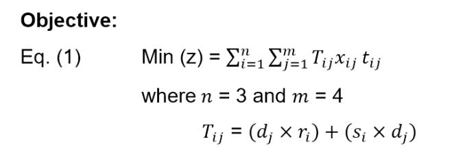
The first objective function of the proposed model given in Eq. (1) minimised the transportation cost of the total orders to each of the assembly lines.

truck fleet optimisation-0d

Cost of delivering the good using truck type  to assembly line  is dependent on the distance travelled to assembly line  based on the rate per distance for the truck and the fuel surcharge per distance to assembly line .

The second objective function proposed model minimises carbon dioxide (CO2) emissions. The second objective function is given in Eq. (2).

truck fleet optimisation-0e

Carbon cost of delivering the good using truck type  to assembly line  is dependent on the distance travelled to assembly line  and the carbon emission rate per KM.

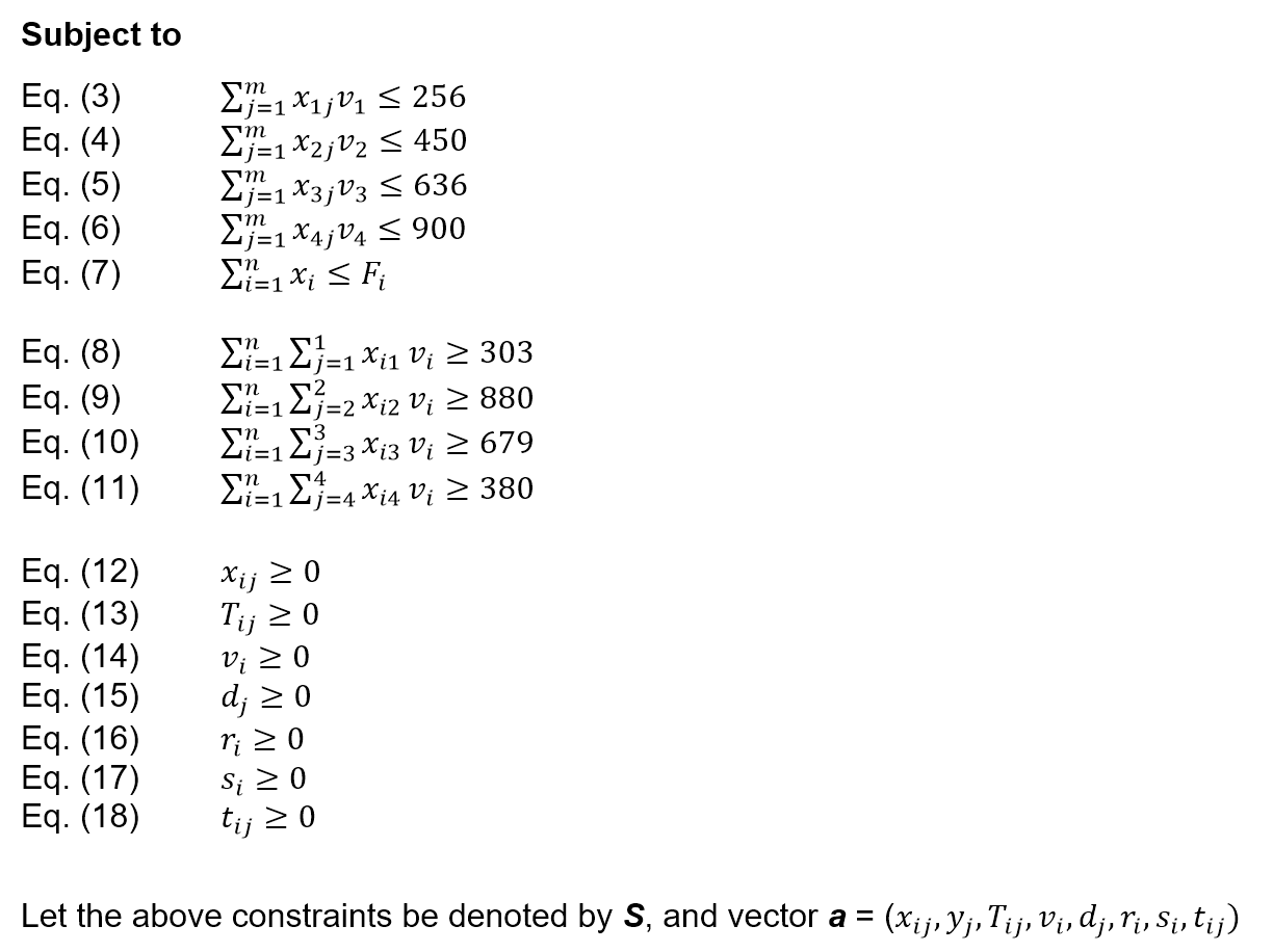
truck fleet optimisation-3

Constraints (3) to (6) determines the maximum supply using each truck types. Eq. (7) ensures that the maximum number of trucks used for each type must be within the fleet x trip size. Eq (8) to (11) determines the maximum demand for each assembly line. Finally, Eq (12) to (18) ensures the non-negativity of variables.

Efficient Frontier Curve

When we solved for both objectives as part of the multi-objective optimisation, we plotted a efficient frontier curve as shown:

truck fleet optimisation-0f

The unusual shape of the frontier curve might be explained by the quadratic cost objective functions as well as the quadratic CO2 emission cost objective function.

But as observed from the chart, the transportation costs are relatively insensitive over the CO2 values over a certain value range; suggesting that unless there is a high penalty cost involved for the ensuring that CO2 emission level is maintained at certain standard, the company is likely to place greater emphasis in minimizing transportation cost and side-line the CO2 emission costs, if there is a need to choose / compromise one objective over the other. In other words, unless CO2 emission cost is high enough, there isn’t an incentive for the supplier to change the fleet configuration so as to further minimise the overall cost of transport and CO2 emissions.

Scenario Testing

We ran multiple scenarios through this model to determine the impact of the various key constraints modelled. The following details the scenarios as well as the interpretation of the results of the LP. The scenarios are detailed in the Transport Data and Matrix.xlsx – Scenarios tab. (refer to Github link below for the xls file)

Scenario: Truck Rental Change

With the reduction on the rental cost of 5 Tons trucks, the supplier should generally maximize on the 5 Tons trucks usage i.e. number of trucks by number of trips. The remaining auto-parts demand that cannot be fulfilled by the 5 Tons trucks are then delivered using either 8 Tons or 10 Tons trucks. However, the changed amount in the scenario might not be significant enough to cause a change in the allocation of supply among the different truck types given the two objectives.

Scenario: Fuel Surcharge Rate Change

With the reduction on the Fuel Surcharge Rate of 5 Tons trucks by 1.2% and an increase for both 8 Tons and 10 Tons truck, the supplier should maximize on the 5 Tons trucks usage i.e. number of trucks by number of trips, which offer benefits on the lower cost form both the truck rental and fuel usage for delivery. The remaining auto-parts demand that cannot be fulfilled by the 5 Tons trucks are then delivered using either 8 Tons or 10 Tons trucks.

Scenario: Fleet Size Change

With the reduction on the number of 5 Ton trucks and an increase in the 8 Ton truck, the supplier should still maximise on the 5 Tons truck usage. However, the remaining auto-parts demand should be allocated to the 8 Ton truck first where possible to benefit on the lower truck rental cost.

Scenario: Volume Change

With the increase in the capacity of 5 Tons truck by 3 cbm, the supplier should maximizes on the 5 Tons trucks usage i.e. number of trucks by number of trips, which offer benefits on the lower cost from both the truck rental with having higher delivery capacity. The remaining auto-parts demands that cannot be fulfilled by the 5 Tons trucks are then delivered using either 8 Tons or 10 Tons trucks.

However, no optimal solution that meet both the objectives can be obtained as no supply can be delivered to assembly line 2. In other words, the demand constraint from assembly line 2 is not met.

Scenario: Demand Change

With an increase in demand from assembly line 1 and line 2 and a decrease in demand from assembly line 3 and 4, it is suggested that we arranged for bigger trucks to fulfil the increased load from line 1 and 2 rather than resort to using more 5 Ton truck.

Scenario: CO2 Adjusted Emission Factor

When there is a change in the carbon dioxide (CO2) adjusted emission factor, the bigger impact is on the carbon dioxide emission cost and not so significant on the transportation cost most of the time. It is probably also dependent on the importance of social corporate responsibility that the supplier has and the penalty cost arising from environmental policy. Technology breakthrough would probably also play a part in moderating the impact of this parameter.

Results

From the scenario analysis, it seems to suggest that the optimisation models here can be used to support the decision making in the company’s new strategy or adapting to new environment factors. For example, the supplier must plan to expand their fleet of truck before they accept any new orders or in anticipation of expanding their business. By stimulating decision variable values for both the demand change and the new fleet size for the various truck types, the supplier can use the information in their decision making when conceptualising their expansion strategy.

I really enjoyed tackling this problem and I hope you have also enjoyed reading this very very long post. But hey, who says optimisation was easy anyway 🙂

You can download the files and play around with the various constraints to explore and see what the results show. All I kindly request is that you make a link back to this post (as an acknowledgement) if you use the code in any of your work or assignments.

Thanks for reading and keep optimising!

A Step by Step How To for Extracting Twitter Messages from R

I recently started a small hobby project to analyse accident frequency on Singapore roads. I decided to extract this information from the Singapore Land Transport Authority twitter feed. (although I could have gotten data through the DataMall initiative by the Singapore Government using Python, this would be the subject of another how-to later  )

I thought I would share my experience and steps to do this and hopefully you will find this useful.

So what are we waiting for? Let’s begin!

Step 1: Download the twitteR package

We need to ensure that the latest twitteR package is installed on your R environment. Run the following command in R Studio

install.packages (twitteR)
This will download and install the twitteR and all required packages.

Step 2: Setup a Twitter App

We need to create a Twitter App so that we can access the Twitter platform through this web API. Before you can create a Twitter App, you need to create an account first. You can do so on the Twitter Apps page.

Once you are done, you can start by clicking on the Create New App button.

Twitter Application Management landing page

Proceed to enter the required mandatory fields as shown below.

Enter required mandatory fields

The Website address can be a temporary one for now. However, ensure that the Callback URL is left blank for now.

Acknowledge the developer agreement and click on the “Create your Twitter application” button. The following page will appear confirming that you have successfully create the web application.

Successfully created a Twitter web application

Click on the Keys and Access Token tab to view the Consumer Key and Consumer Secret keys.

View keys and access tokens

At this point, you have not created your Access Token yet. Hence click on “Create my access token” button to do so.

Create access token
Create access token

Your access tokens will be generated and displayed on the refreshed page.

Access token generated

Click on the Application Management icon above and you will see your new application created as shown below.

Twitter application successfully created

Step 3: Create R code to Access Twitter Feeds

Go back to RStudio and enter the following R code:

#install the necessary packages
library(twitteR)

#necessary file for Windows
#download.file(url="http://curl.haxx.se/ca/cacert.pem", destfile="cacert.pem")

#to get your consumerKey and consumerSecret see the twitteR documentation for instructions
consumer_key <- 'your consumer key'
consumer_secret <- 'your consumer secret key'
access_token access_secret <- 'your access secret’

setup_twitter_oauth(consumer_key, consumer_secret, access_token, access_secret)

Note that I have commented out the download.file command since I am running OS X in this example. I have not tested whether adding this download.file(…) code snippet will work.

Once you have entered the above, run the code and you will see the following prompt on the RStudio console

Running R code for twitter integration

You can select 1 or 2 depending on your preference. Regardless of the choice, you should see the “>” on the next line on the console indicating that the setup_twitter_oauth command was successfully executed.

Step 4: Extract your Twitter Feed

Once you have completed the above step, enter the following R code.

ltaTwtr <- searchTwitter("LTATrafficNews + Accident", n=500)
length(ltaTwtr)

#make data frame
tmpDf <- do.call("rbind", lapply(ltaTwtr, as.data.frame))

The command searchTwitter will issue a search of Twitter based on a supplied search string – based on your subscribed twitter feeds. Because the return value of searchTwitter is a list, we would need to do.call(“rbind”…) function to convert it into a data frame for subsequent processing.

Data from twitter feed based on search string

The above table is an example of the twitter messages that match my search criterion.

That’s it!

You can download my sample code on Github for those who want the code directly.

I hope this short how-to has help with your data science tasks! Happy coding!

What is analytics? A quick dip in the pool.

I came across this great visualisation that introduces basic concepts in analytics and the differences between Big Data and predictive analytics. I found this to be a good summary for the busy senior executive who wants to understand what analytics is all about.

Most certainly there is so much more to analytics than just this summary – but its a good dip in the water! 🙂

http://www.microsoft.com/en-gb/enterprise/it-trends/big-data/articles/getting-started-with-predictive-analytics.aspx?linkId=15086654#fbid=mq4jQRs-uCm

Thanks to Jesse Stanchak, Social Media Community Manager @ Microsoft!